Roads
Roads Default model
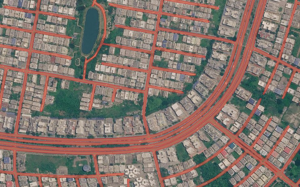
Example result: road polygons built from a cleaned centreline network.
Cost
5 credits per km² + imagery
Example: 10 km² on Mapbox zoom 18 ≈ 80 credits.
Finds road centrelines, cleans the graph (simplifies geometry, merges gaps, removes double edges and short detached pieces) and turns it back into road polygons. Multi-task learning keeps the network connected where trees or buildings hide the road.
What you get
Road polygons built from a cleaned centreline network.
Works best with
Rural and suburban areas with 0.6–0.3 m imagery (zoom 18). Dense city centres with wide sidewalks and complex crossings are harder.
Usage examples
Map access roads and tracks for rural planning
Add forestry and field tracks missing from OSM
Check the street network in new suburbs
- Version
1.1
- Geo domain
Global, best in rural and suburban areas
- Method
Segmentation + graph post-processing
- GSD / zoom
0.6–0.3 m / z18
How it works
The model is trained mostly on rural and suburban areas. Multi-task learning keeps the road mask connected where trees or buildings hide the road. It can fail in cities with wide roads, sidewalks and complex crossings.
The model extracts road centrelines to reduce clutter, cleans the network, then inflates the lines back into road polygons. Since version 1.1 the road graph is post-processed:
geometry simplification;
merging of gaps;
removal of double edges;
removal of detached and too short segments.
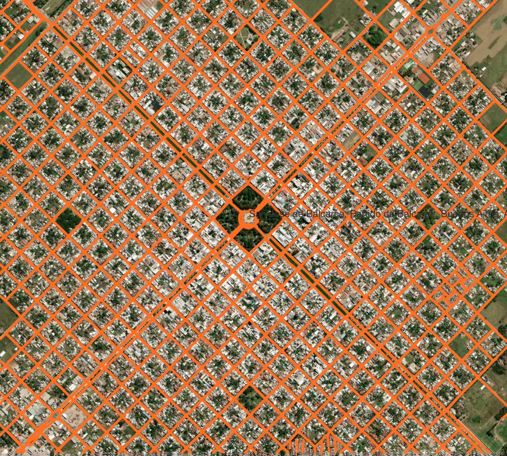
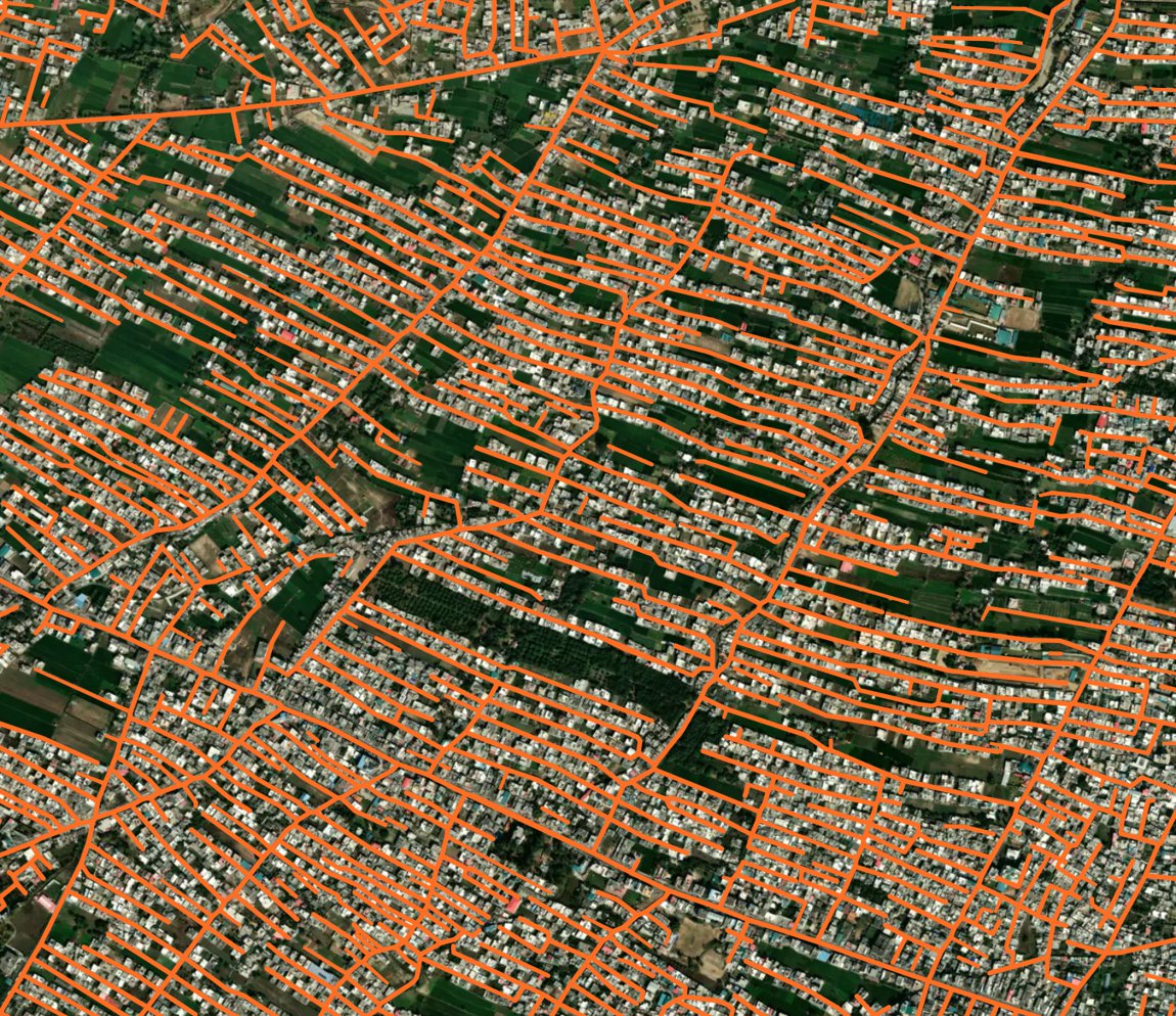
Sample results
📊 Benchmarks
We evaluated the update using open benchmark datasets, including SpaceNet 3 Roads, supplemented with our own validation data across different urban environments.
We focused on two complementary metrics:
IoU (Intersection over Union) measures how accurately the predicted road mask matches the actual road coverage. It tells us how well the model identifies roads and captures their spatial extent.
Topology F1 (Topo-F1) evaluates the connectivity of the extracted road network. This is particularly important for mapping and routing, where roads need to remain connected even when partially obscured by vegetation, buildings or shadows.
The new model improves both metrics across all seven validation datasets. Compared with the original baseline, the average scores across these datasets increased significantly:
IoU: 0.386 → 0.599 (+55%)
Topo-F1: 0.465 → 0.758 (+63%)
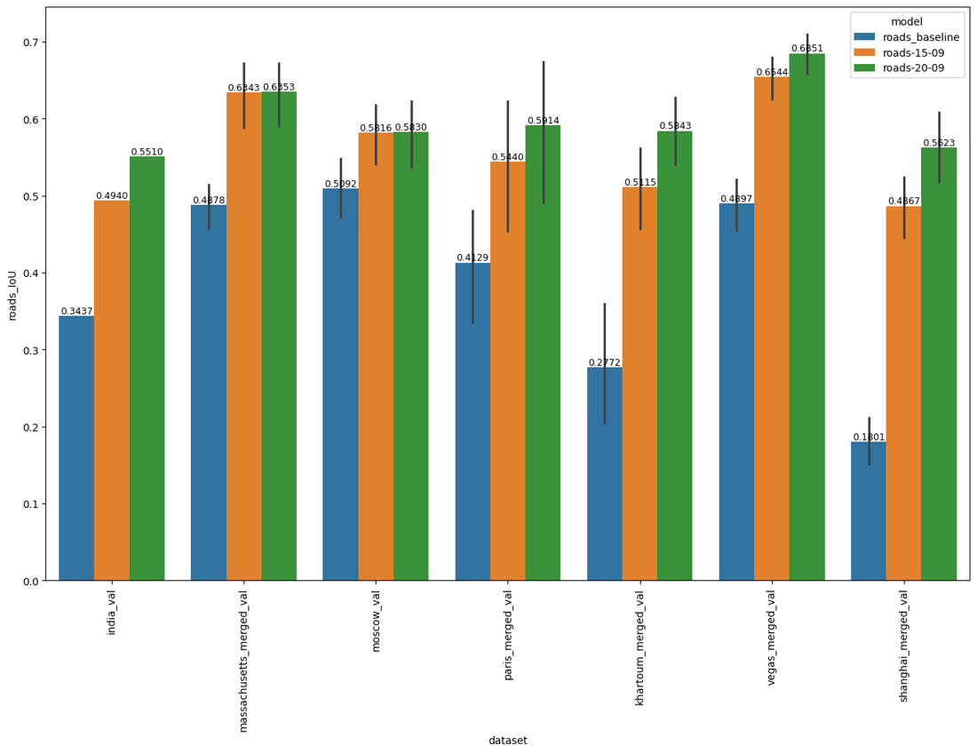
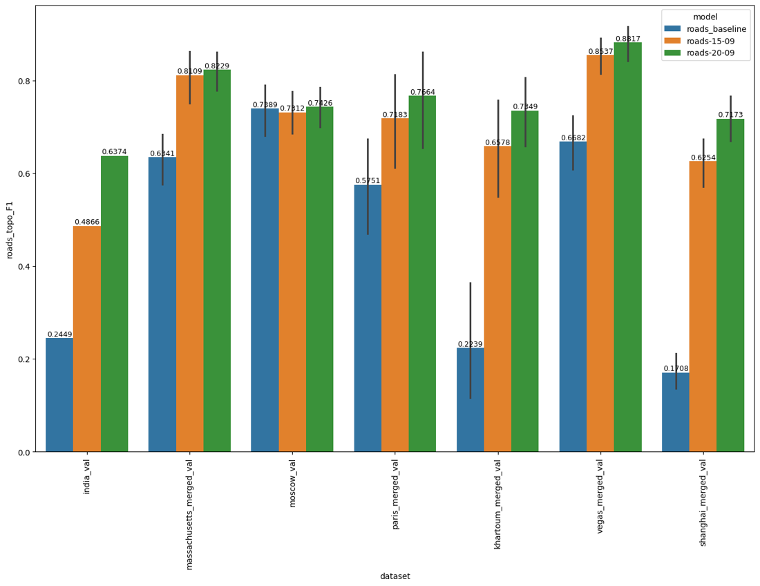
Some of the most impressive improvements are in challenging urban environments:
Validation area |
IoU (before → after) |
Topo-F1 (before → after) |
|---|---|---|
Shanghai |
0.180 → 0.562 |
0.171 → 0.717 |
Khartoum |
0.277 → 0.584 |
0.224 → 0.735 |
India |
0.344 → 0.551 |
0.245 → 0.637 |
Las Vegas |
0.490 → 0.685 |
0.668 → 0.882 |
Why do both metrics matter?
A road network may look connected but still miss substantial portions of the actual road coverage. Conversely, a model can accurately identify individual road segments but fail to connect them into a usable network.
The updated Roads model makes progress on both fronts: more accurate road coverage and better-connected networks. This is especially valuable in densely built-up areas with narrow streets, irregular layouts and frequent occlusions — precisely where automated road mapping remains challenging.
Need a different object?
We train custom models on your imagery and classes, and connect them to your Mapflow account.